Simulating an Ideal Radio Interferometer

In radio interferometry, an ideal radio interferometer is assumed to provide full \((u,v)\) coverage for a given resolution. We have implemented a method in the Observation class that allows the simulation of such an interferometer; mostly relying on calc_dense_baselines(). The type of \((u,v)\) grid that we will use in the following is referred to as dense grid, where \((u,v)\) data is distributed as densely as is necessary to obtain an ideal \((u,v)\) coverage.

In the following sections, we will cover how pyvisgen simulates an ideal radio interferometer:

Note

The code shown in this example does not contain the funtions used for plotting. To view the full code, please have a look at this Jupyter Notebook.

1. Creating an Example Image

Essential imports

  import numpy as np
  from numpy.fft import ifft2, fftshift

  import matplotlib.pyplot as plt
  from matplotlib.colors import LogNorm, CenteredNorm

  from scipy.constants import c
  from scipy.stats import gaussian_kde

  import torch
  from pytorch_finufft.functional import finufft_type1 as nufft2

  import h5py

  device = "cuda:0" # use GPU, change to "cpu" if no GPU available

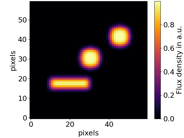
Test image in real space assumed as the true sky flux density distribution.

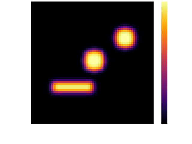
Test image in real space assumed as the true sky flux density distribution.

The figure above is the test image in real space we will assume as our real sky flux density distribution. Additionally we require the following parameters for our simulated observation:

Parameter	Variable	Value	Unit	Explanation
Image Size	img_size	60	pixel	The side length of the test image
Frequency	freq	230	GHz	The frequency we observe the source at
Field Of View	fov	6000	arcsec	The Field Of View of the test image

Define the preset values and import model image.

img = h5py.File("test_model.h5", "r")["model"][()] # import the test model
img_size = img.shape[0] # 60

fov = 6000  # fov in asec
freq = 230e9  # Frequency in Hz
wavelength = c / freq

2. Creating the Ideal \((u,v)\) Coverage

For the ideal coverage, we want to create exactly one \((u,v)\) point in each pixel of the image in Fourier space. To achieve this, we first have to consider the physical size of one pixel in Fourier space. We will name this quantity delta_uv, i.e. the pixel size in \((u,v)\) space. This is calculated as the reciprocal value of the fov in the unit radians.

delta_uv is computed from the fov (first converted from arcsec to degrees, then to radians). Mutliplying that value with the wavelength yields the physical size of one pixel.

delta_uv = np.deg2rad(fov / 3600) ** (-1) # fov / 3600 to convert from asec to deg
delta_uv *= wavelength

Multiplying delta_uv with the wavelength of the observation yields the physical pixel size in Fourier space.

To create a grid of \((u,v)\) points, we will have to create two linear axes: one for \(u\) and one for \(v\). Since the scale of both is the same, we will only create one and copy it to the other one. Additionally we want their values to be in the center of their respective pixel. This means that one pair should be exactly at the Coordinate \((u,v) = (0, 0)\). To achieve this, we will also have to choose our binning correctly later on. Since every pixel should contain one point, we can simply use numpy.arange to create our \(u\) and \(v\) axes. From these we can then create a 2-dimensional grid using numpy.meshgrid.

uu = (np.arange(
    start=(-img_size / 2) * delta_uv,
    stop=(img_size / 2) * delta_uv,
    step=delta_uv, dtype=np.float128)
    ).astype(np.float64)

vv = np.copy(uu)

uv_grid = np.meshgrid(uu, vv)

The values are in the range from

(1)\[\begin{equation} \left[-\frac{N_{\text{image}}}{2} \cdot \delta_{uv},\,\frac{N_{\text{image}}}{2} \cdot \delta_{uv}\right] \end{equation}\]

where \(N_{\text{image}}\) is img_size and \(\delta_{uv}\) is delta_uv. This means that there will be zero values for our Fourier space coordinates and we will have as many coordinates as we have pixels.

Note

The grid is created using the data type float128 since the magnitude of the delta_uv values can differ severly depending on the choice of the Field Of View and the size of the image. For small values of the fov and small images this is not as much of a problem, but for large values the precision of the default float64 data type leads to major instabilites and non-linearities which alter the grid and therefore the simulation. The usage of the larger data type ensures that the axes are equidistant. This equidistance it preserved when casting the array to float64.

It is not optional to cast the type back to the 64-bit variant, since the simulation runs using pytorch which does not support the float128 data type.

To picture ourselves where these points will be in the grid our pixels create, we will have to create a binning that creates quadratic bins with exactly one pixel per bin. These will be used to create the gridded \((u,v)\) after we calculated the visiblities. These bins will have the same width and heigth as our pixels but since we will create the edges of the bins, there will be one value more on each axis then there are \(u\) and \(v\) values. This can be achieved by adding an offset of half a pixel size (delta_uv) in each direction along the axis.

  bins = (np.arange(
      start=-(img_size / 2 + 1/2) * delta_uv,
      stop=(img_size / 2 + 1/2) * delta_uv,
      step=delta_uv,
      dtype=np.float128))

This positions the bin edges exactly half a delta_uv left and right of the points so that every 2-dimensional bin contains exactly one point.

These points can now be plotted in the created grid with the following code:

fig, ax = plt.subplots(1, 1, figsize=(10, 10))
for b in bins:
    ax.axvline(x=b, color="black")
    ax.axhline(y=b, color="black")

ax.scatter(uv_grid[0], uv_grid[1], s=10, color="royalblue")
ax.set_xlabel("$u$ in $\\lambda$")
ax.set_ylabel("$v$ in $\\lambda$")

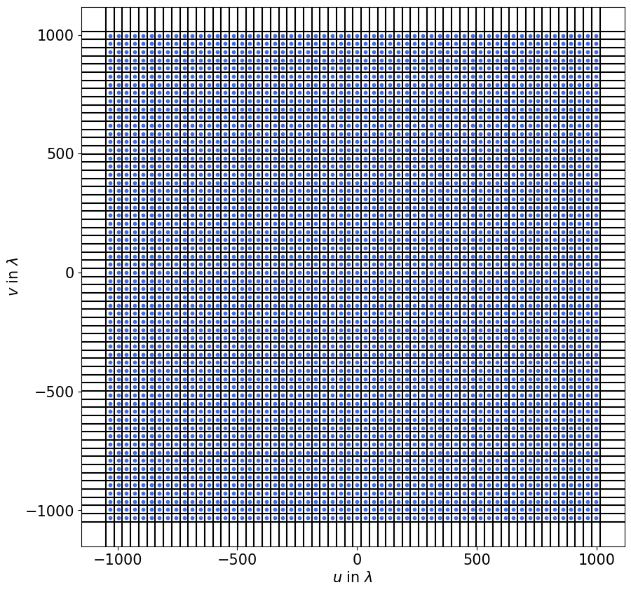
\((u, v)\) grid.

\((u, v)\) grid.

Since this seems to be working, we can now proceed to combine our generated \((u,v)\) coverage and our image.

3. Simulating the Observation

The next step is to calculate the visiblities our interferometer measures. To do this we need to use the RIME formalism as described by Smirnov [Smi11], which uses a Jones formalism to model the path of the radio signal using a sum of matrix multiplications. The full-sky RIME is given by the following fomula:

(2)\[\begin{equation} V_{pq}(u_{pq}, v_{pq}) = \int_l\int_m \mathrm{\overline{E}}_p(l, m)\mathrm{K}_p(l, m) \mathrm{B}(l, m) \mathrm{K}_q^\dagger(l, m)\mathrm{\overline{E}}_q^\dagger(l, m) \frac{\symup{d}m\;\symup{d}l}{n} \end{equation}\]

The 2-dimensional intensity distribution of the observed source, in our case our test image, is described by the \(\mathrm{B}\) matrix. We integrate over the direction cosines \(l\) and \(m\), which describe the position of the source on the tangential plane projection of our sky. Since the telescopes \(p\) and \(q\) are at seperate positions, the signal arrives with a geometrically based time delay between them. This creates a phase delay between the received signals. This is described by the \(\mathrm{K}_{p, q}\), which are combined by multiplication to form the \(\mathrm{K_{pq}}\) matrix, which takes the form

(3)\[\begin{equation} K_{pq} = \exp\left[-2\pi i\left( u_{pq} l + v_{pq} m + w_{pq}\left(\sqrt{1 - l^2 - m^2} - 1\right)\right)\right] \end{equation}\]

There our \(u\) and \(v\) coordinates are used to describe the positions of the telescopes normalized to the wavelength of our signal wave. The \(\mathrm{\overline{E}}\) matrix describes the direction dependent effects of the telescope response. It is convention to define the \(w_{pq}\) dependent part of the \(\mathrm{K}\) matrix and the \(1/n\) into the \(\mathrm{\overline{E}}\) matrix which then becomes the \(\mathrm{\overline{E}}\) matrix. Since we are looking at a perfect interferometer, we assume that we can neglect direction dependent effects which means that \(\mathrm{E} = \mathbb{1}\).

This means that our needed equation to describe the visiblities of a pair of telescopes \(pq\) looks like this:

(4)\[\begin{equation} \mathrm{V}_{pq}(u_{pq},v_{pq}) = \int_l\int_m \mathrm{B}(l,m) \exp\left( -2\pi i \left( u_{pq}l + v_{pq}m \right)\right) \symup{d}m\;\symup{d}l \end{equation}\]

This is nothing less but the 2-dimensional Fourier transform of our model intensity distribution. Since we are in a discrete case, since our distribution is divided into pixels, the integral transitions to a discrete sum over the \((l, m)\) coordinates of each pixel.

What’s special about this Fourier transform is, that the real space coordinates are not equidistant. This is a problem if one is using a typical Fast Fourier Transform (FFT) algorithm like numpy.fft.fft since these assume a homogenous real space. For this reason we will have to use a Nonuniform Fast Fourier Transform (NUFFT) like the python implementation FINUFFT by the Flatiron Institute Barnett et al. [BMaK19].

In this the following formula is used to calculate the 2-dimensional Fourier transform for nonuniform coordinates:

(5)\[\begin{equation} f_{kl} = \sum_{i, j=1}^M c_{ij} e^{i (kx_j + ly_i)}~, \qquad \mbox{ for } \; k, l\in\mathbb{Z}, \quad -N/2 \le k,l \le N/2-1 ~. \end{equation}\]

If we look at their coefficients, we can see, that we will need to modify our \((l, m)\) coordinates, since they are the \(x\) parameters in this transform. Because the formula assumes the Fourier space coordinates \((k, l)\) to be whole numbers, we will need to put their scaling (the scaling of \((u, v)\)) into our \((l, m)\) coordinates as well. The formula also assumes the real space coordinates to be a manifold of \(2\pi\), which means this we will have to move into our coordinates as well.

All in all we end up with the substitution:

(6)\[\begin{equation} (x_i, y_j) = (l, m) \to \frac{2\pi}{\Theta}(l, m), \end{equation}\]

with \(\Theta\) being the Field of View. Since the calculations of pyvisgen are done using pytorch to enable GPU-based calculations, we will use the FINUFFT wrapper pytorch-finufft.

To perform this calculation in our code, we will first need to create the values of \((l, m)\). These are the direction cosines of a uniform grid in an equatorial coordinate system with coordinates RA (Right Ascension) and DEC (Declination). This grid will be called rd_grid. The code to calculate this grid is taken from create_rd_grid() and create_lm_grid().

def create_rd_grid(fov, img_size, dec):
    res = fov / img_size
    r = torch.from_numpy(
        np.arange(
            start=-(img_size / 2) * res,
            stop=(img_size / 2) * res,
            step=res,
            dtype=np.float128,
        ).astype(np.float64)
    ).to(device)
    d = r + dec

    R, _ = torch.meshgrid((r, r), indexing="xy")
    _, D = torch.meshgrid((d, d), indexing="xy")
    rd_grid = torch.cat([R[..., None], D[..., None]], dim=2)

    return rd_grid

def create_lm_grid(fov, img_size, dec):

    dec = np.deg2rad(dec).astype(np.float128)

    rd = create_rd_grid(fov=fov,
                        img_size=img_size,
                        dec=dec).cpu().numpy().astype(np.float128)

    lm_grid = np.zeros(rd.shape, dtype=np.float128)
    lm_grid[..., 0] = np.cos(rd[..., 1]) * np.sin(rd[..., 0])
    lm_grid[..., 1] = np.sin(rd[..., 1]) * np.cos(dec) - np.cos(
        rd[..., 1]
    ) * np.sin(dec) * np.cos(rd[..., 0])

    return torch.from_numpy(lm_grid.astype(np.float64)).to(device)

We will assume that the center of our model is located at the declination \(0\;\symup{deg}\).

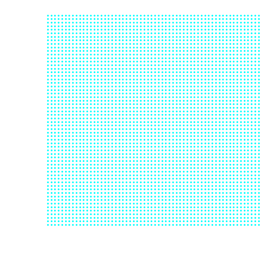
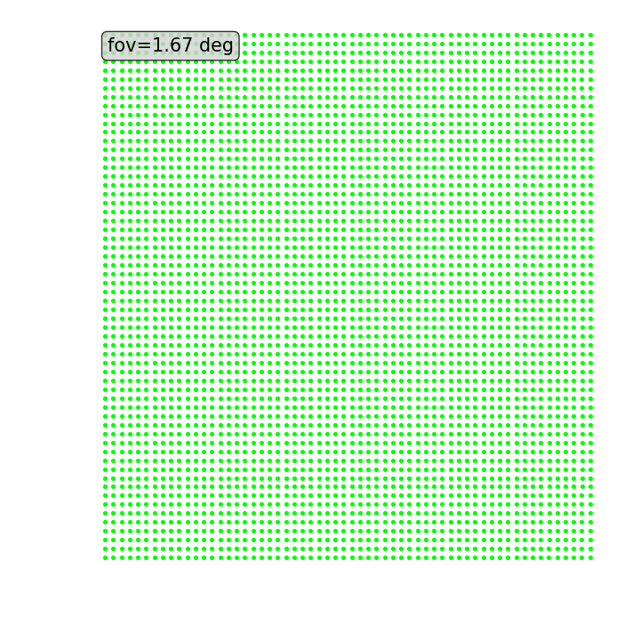
To demonstrate the effect of the non-equidistant \((l, m)\) points, we will first look at a much larger section of the sky with a FoV of \(90\;\symup{deg}\).

    test_grid = create_lm_grid(fov=np.deg2rad(90), img_size=img_size, dec=0)

The created \((l, m)\) grid is shown in the figure below.

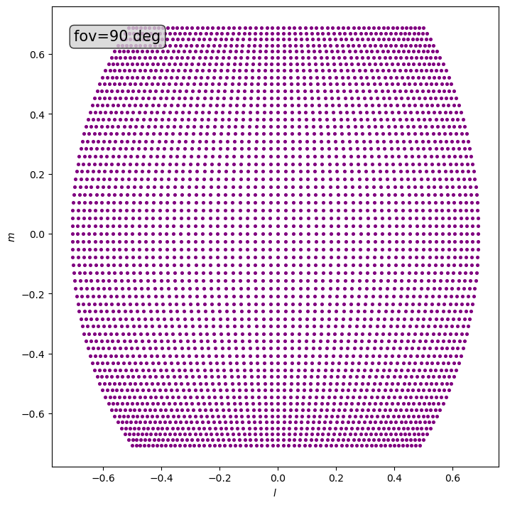
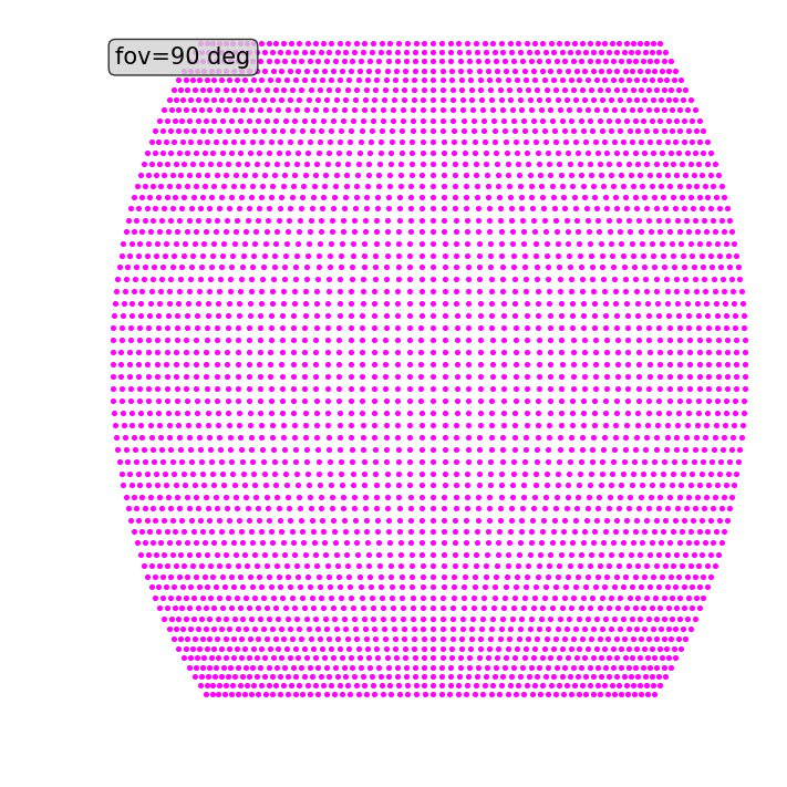
We can clearly see that the grid is not homogenous on the \(l\) and the \(m\) axes. This effect is existent but less impactful in case of a small FoV.

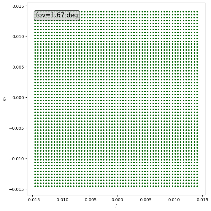
The correct grid with our Field of View is calculated and plotted below:

    lm_grid = create_lm_grid(fov=fov, img_size=img_size, dec=0)

    l = lm_grid[..., 0, 0].cpu().numpy()
    m = lm_grid[..., 1, 0].cpu().numpy()

Now that we have our \((l, m)\) grid set up, we can continue to calculate the nonuniform Fourier transform:

    x = 2 * torch.pi * lm_grid[..., 0].flatten() / fov
    y = 2 * torch.pi * lm_grid[..., 1].flatten() / fov

    img_flat = torch.tensor(img, dtype=torch.complex128)
    img_flat = img_flat.to(device).flatten() # send to GPU and transform image to vector

    stokes_i = nufft2(points=torch.vstack([x, y]),
                      values=img_flat,
                      output_shape=(img_size, img_size),
                      isign=-1,
                      eps=1e-15).cpu().numpy() # compute nonuniform FFT

We will call our Fourier transformed image stokes_i since it is the \(I\) component of the Stokes matrix of the source distribution.

Since we have a perfect grid, we would be able to just plot our results straight away, but since we want to check, if our \((u, v)\) grid was created correctly, we will proceed to perform the regular gridding process, we would also use, if the \((u, v)\) coordinates were generated by a measurement.

The gridding works analogously to that in the Gridding module. In short, it matches of \((u, v)\) coordinates and corresponding visibility values to create the samps. The \((u, v)\) coordinates are then assigned to the same 2d grid, we created earlier by creating a 2-dimensional histogram with the stokes_i values as weights (real and imaginary parts of the visiblities are put in individual histograms).

    real = stokes_i.real.T
    imag = stokes_i.imag.T

    samps = np.array(
        [
            np.append(-uv_grid[0].ravel(), uv_grid[0].ravel()),
            np.append(-uv_grid[1].ravel(), uv_grid[1].ravel()),
            np.append(real.ravel(), real.ravel()),
            np.append(-imag.ravel(), imag.ravel()),
        ]
    )

    mask, *_ = np.histogram2d(samps[0], samps[1], bins=[bins, bins], density=False)
    mask[mask == 0] = 1

    mask_real, x_edges, y_edges = np.histogram2d(
        samps[0], samps[1], bins=[bins, bins], weights=samps[2], density=False
    )
    mask_imag, x_edges, y_edges = np.histogram2d(
        samps[0], samps[1], bins=[bins, bins], weights=samps[3], density=False
    )
    mask_real /= mask
    mask_imag /= mask

    dirty_img = np.abs(fftshift(ifft2(fftshift(mask_real + 1j * mask_imag))))

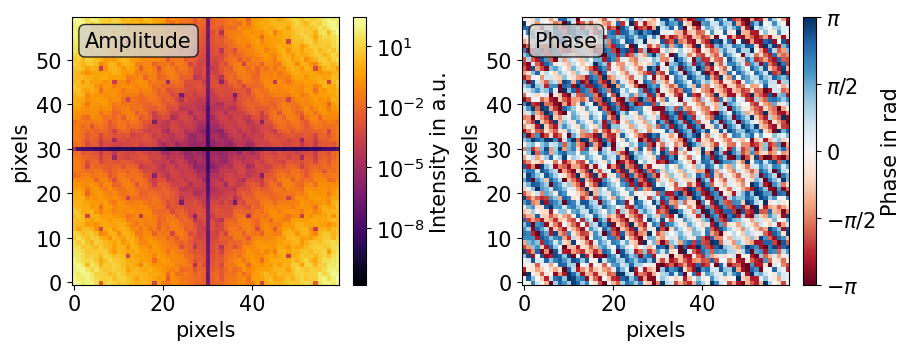
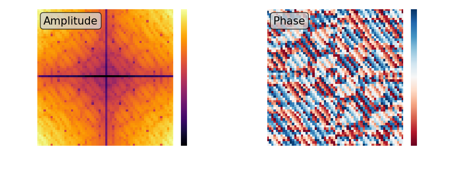
These histograms with the real and imaginary parts of the visibilities can then be plotted in a regular image. Since we are obviously dealing with complex numbers, we will have to split the visibility masks in either real and imaginary or in this case in amplitude and phase according to Eulers formula:

(7)\[\begin{equation} c = a\cdot \exp(i\varphi),\;\; c \in \mathbb{C}. \end{equation}\]

The two resulting components are shown below.

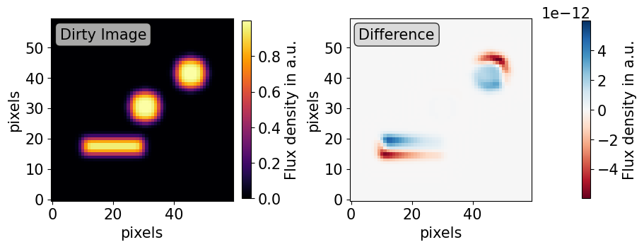
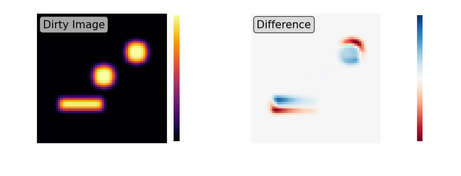
Finally we can look at our resulting “dirty” image. Since we have a perfect \((u, v)\) coverage, we can hardly call this “dirty” but it was created just like an image with incomplete coverage. Additionally to the dirty image, we can also calculate the difference between the dirty image and the model.

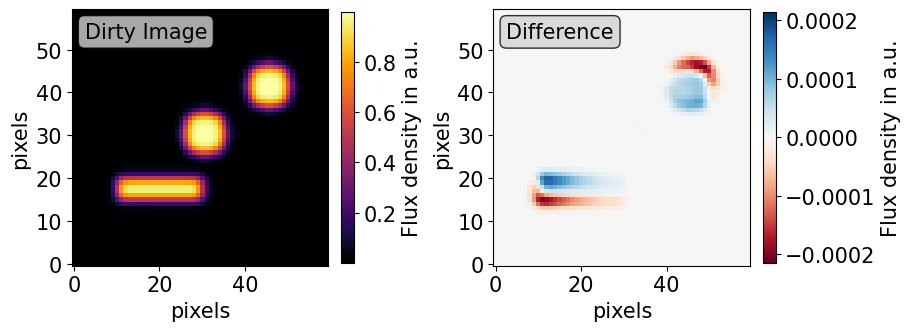
We can clearly see, that the \((l, m)\) grid, that was assumed as the real space coordinates, caused a distortion. This distortion depends on the physical size of the part of the sky we are looking at. The distrotion of the coordinates becomes much more visible, meaning the difference becomes greater, the larger we make the Field of View of our image. Since we used an FoV of \(6000\;\symup{asec}\), we can clearly see the distortion in a significant intensity, while an image with smaller FoV won’t be affected as much by the effect.

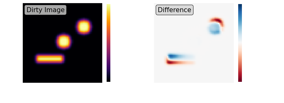
The below image is simulated with an FoV of \(1\;\symup{asec}\) and the difference between dirty image and model is only visible in a magintude of \(10^{-12}\), which is way below a realistically achievable sensitivity of a real measurement.